Bellman-Ford Algorithm

History of Bellman-Ford Algorithm:

Alfonso Shimbel suggested this algorithm in 1955, however it was named after Richard Bellman and Lester Ford Jr., who published it in 1958 and 1956, respectively. In 1959, Edward F. Moore published a variant of the algorithm, which is often referred to as the Bellman–Ford–Moore algorithm. Leaving about the history lets quickly jump into the topic.

Basic Overview on Bellman-Ford:

The problem is, in a directed weighted graph we have to select one of the vertex as the source vertex and find the shortest path to all other vertices. For doing this we have Dijkstra algorithm that solves shortest path problem. But the problem here is Dijkstra algorithm will not work with negative edges, it may or may not give correct answer. So, we need an algorithm which confirms the answers are correct, that is called Bellman-Ford algorithm. The Bellman-Ford algorithm is a very popular algorithm used to find the shortest path from one node to all the other nodes in a weighted graph. It also simpler than Dijkstra algorithm and more versatile. Similar to Dijkstra’s Algorithm, it uses the idea of relaxation but doesn’t use with greedy technique. It is based on the “Principle of Relaxation”. It follows Dynamic programming. So, we try all possible solutions and pick out best solution. This blog explains the pros and cons of Bellman-Ford algorithm.

Analysis of Bellman-Ford Algorithm:

Pseudo code:

function BellmanFord(list vertices, list edges, vertex source) is

// This implementation takes in a graph, represented as

// lists of vertices (represented as integers [0..n-1]) and edges,

// and fills two arrays (distance and predecessor) holding

// the shortest path from the source to each vertex

distance := list of size n

predecessor := list of size n

// Step 1: initialize graph

for each vertex v in vertices do

distance[v] := inf // Initialize the distance to all vertices to infinity

predecessor[v] := null // And having a null predecessor

distance[source] := 0 // The distance from the source to itself is, of course, zero

// Step 2: relax edges repeatedly

repeat |V|−1 times:

for each edge (u, v) with weight w in edges do

if distance[u] + w < distance[v] then

distance[v] := distance[u] + w

predecessor[v] := u

// Step 3: check for negative-weight cycles

for each edge (u, v) with weight w in edges do

if distance[u] + w < distance[v] then

error “Graph contains a negative-weight cycle”

return distance, predecessor

Explanation:

1)In a directed graph we initially consider distances from the source to all vertices as infinite and distance to the source itself as 0.

2) if there are two vertices (u,v) if the distance of u and weight of an edge (u,v) is less than distance of v then change the distance of vertex v to sum of distance of u and weight of an edge (u,v).We go on relaxing all the edges for V-1 times(V is vertices) , and make sure all the vertices are covered.

3) It checks whether the negative cycle exist in graph. Doing this for each edge u-v and if d[v] > d[u] + w(u,v) even after |V|-1 iterations then there is negative weight cycle.

4) After |V|-1 iterations there shall be no chance of changing the distance of nodes.

Time Complexity:

· The first step takes O(V) time.

· Then, it iterates (|V|-1) times, where each iteration taking O(1) time.

· After (|V|-1) interactions, it chooses all the edges and then passes all the edges to Relax(). Choosing all the edges takes O(E) time and the function Relax() takes O(1) time.

· So, to complete all the operations it takes O(VE) time.

· i.e., O(n²) (considering V and E as n).

· If the graph is complete graph i.e., there is an edge between every pair of vertices. So total number of edges |E|=n(n-1)/2. So, the time complexity becomes O(n³).

· So, we can conclude that in worst case time complexity is O(n³) and average case O(VE) time.

Why does it fails for Negative cycles :

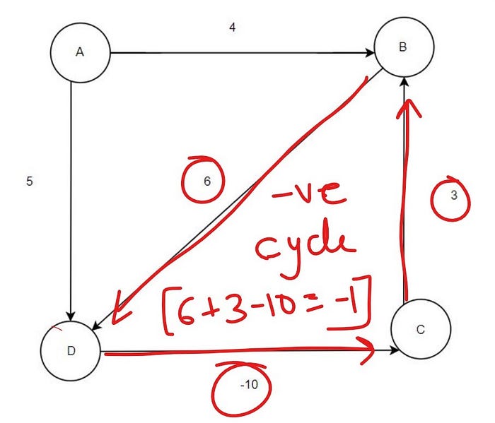
It’s because Bellman ford Relaxes all the edges. It finds a global optimum solution and so if there is a negative cycle, the algorithm will keep ongoing indefinitely. It will always keep finding a more optimized, that is, a more negative value than before.

Applications of Bellman-Ford Algorithm:

» Networks (Routing )

Ex1: Google map may use Bellman-Ford algorithm for finding shortest path between locations: 1) Consider map as graph 2)locations in the map are our vertices. 3) Roads and road lengths between locations are edges and weights.

Ex2: Consider the following scenario: you need to get to a baseball game from your home. One of two things can happen along the way, on each lane. To begin with, the road you’re on may be a toll road, and you may be required to pay a fee. Second, you might know someone who lives on that street (like a family member or a friend). Those people might be willing to lend you money to help you replenish your wallet. You need to get across town, and you want to arrive with as much cash as possible in order to buy hot dogs. You can use Bellman-Ford to help plan the best optimal route if you know which roads are toll roads and which roads have people who can lend you money.

» Robot Navigation

» Urban Traffic Planning

» Telemarketer operator scheduling

» Routing of Communication messages

» Optimal truck routing through given traffic congestion patteren.
» OSPF routing protocol for IP

Advantages:

Bellman-ford finds the shortest path between pair of vertices even if there is negative weights between the nodes.

It also simpler than Dijkstra algorithm and more versatile.

This algorithm is simple and it does not need any complex data structures and can find the minimum path weight with high efficiency and accuracy.

Since it follows Dynamic programming It is guaranteed that it will generate an optimal solution using Principle of Optimality.

Bellman-Ford works better (better than Dijkstra’s) for distributed systems. Unlike Dijkstra’s where we need to find the minimum value of all vertices, in Bellman-Ford, edges are considered one by one.

Drawbacks:

In a graph if there is a cycle of edges and total weight of that cycle is negative then graph cannot be solved by Bellman-Ford algorithm.

Time complexity is more than Dijkstra algorithm with respect to time

The Bellman-Ford algorithm deals more effective with small number of nodes, and the Dijkstra algorithm is more efficient for a large number of nodes.

Conclusion:

So far, we have discussed about Bellman-Ford Algorithm, I hope this article made clear about the topic. Try this algorithm with an example then you can understand it in a better way.

Thank you.

Happy Coding😊

“Eat Sleep Code🤗”